PAM Representation of GMSK and Serial Receivers

1. Abstract

This report is on Laurent Representation (a.k.a. PAM representation) of GMSK. According to Laurent, a CPM signal can be written as sum of several PAM signals. Laurent's representation of CPM signals resembles Fourier decomposition in many ways. This approach enables many different receiver types, most notably the serial receiver, which is found by Kaleh.

You can find sample MATLAB codes here.

2. Introduction

GMSK waveform is a CPM scheme and can be modeled as sum of several PAM waveforms [1]. Luarent's representation enabled two new receivers for CPM signals, especially for GMSK [2, 3]. First one is a Viterbi Algorithm type of receiver and the second one is a serial receiver. Since there are other, easier to understand and implement Viterbi Algorithm receivers for GMSK, this one is not further investigated in this report. However, the computation cost of the serial receiver is very low, which is why this report is written.

In the following section, mathematical background of PAM representation of CPM is further investigated. After that a sample problem is solved for a specific case for further clarification of the subject. Next, some remarks are reiterated for clarification of PAM representation. Finally, the serial receiver is implemented and simulation results are presented.

3. PAM Representation of CPM

A CPM signal has the following form [4]:

s(t, \underline{\alpha}) = \sqrt{\frac{E}{T}}exp\{j\psi(t, \underline{\alpha})\},

where E is the symbol energy, T is the symbol duration and \underline{\alpha} is a sequence of bipolar NRZ symbols. \psi(t, \underline{\alpha}) is defined as follows:

\psi(t, \underline{\alpha}) = \pi h\sum_{i=0}^{n} \alpha_i q(t-iT), \quad nT \leq t < (n+1)T.
Here, h is the modulation index and is always 0.5 for MSK signals. q(\cdot) is the so called phase shaping filter:

q(t) =
\begin{cases}
0, & t < 0, \\ \int_{0}^{t}f(\tau)d\tau, & 0 \leq t < LT,\\ 1, & t \geq LT \end{cases}
where f(\cdot) is the frequency shaping filter. It is defined as follows:

f(t) = \frac{1}{2T}\bigg[Q(2\pi B \frac{t-\frac{T}{2}}{\sqrt{ln(2)}}) - Q(2\pi B \frac{t+\frac{T}{2}}{\sqrt{ln(2)}})\bigg],

where B = BT/T, with BT the so called time bandwidth product Q(\cdot) is the famous Q function.

Laurent rewrote Eq. eq:cpm_sig}:

s(t, \underline{\alpha}) = \sqrt{E}\sum_{k=0}^{2^{L-1}} \sum_{i=0}^{n-1} a_{k,n} h_k(t-nT),

where L is the extent of the phase shaping function as in Eq. eq:phase_shaping, a_{k,n} are the so called auxiliary symbols. Finally h_k(\cdot) is the PAM signal and is different from the modulation index h.

In order to formulate h_k(\cdot) Luarent started with two auxiliary equations [1]:

J \triangleq e^{jh\pi},

and

c(t) \triangleq \begin{cases}
\frac{sin(\pi h - \pi h q(t))}{sin(\pi h)}, & 0 \leq t < LT, \\ c(-t), & -LT < t \leq 0, \\ 0, & o.w. \end{cases}
with h being the modulation index in both equations. Then the exponential part in Eq. eq:cpm_sig is rewritten as follows:

exp\{j\psi(t, \underline{\alpha})\} = exp\bigg\{j\pi h\sum_{i=0}^{n-L} \alpha_i \bigg\} \prod_{i=n-L+1}^{n} exp\big\{j\pi h\alpha_i q(t-nT)\big\}.

This is very much like the Trellis like representation in [5]. Since for MSK, h=0.5, Eq. eq:c_long can be simplified as follows:

c(t) \triangleq \begin{cases}
cos\Big(\frac{\pi q(t)}{2}\Big), & 0 \leq t < LT, \\ c(-t), & -LT < t \leq 0, \\ 0, & o.w. \end{cases}
In addition to this, in MSK \alpha_i are bipolar NRZ, s.t. \alpha_i \in \{\pm1\}. Thus J^{\alpha_i} = cos(\pi h) + j\alpha_i sin(\pi h). This is a direct consequence of \alpha_i being bipolar NRZ.

The product term in Eq. eq:rewrite becomes:

exp\big\{j\pi h\alpha_i q(t-nT)\big\} = cos\big(\pi h\alpha_i q(t-nT)\big) +jsin\big(\pi h\alpha_i q(t-nT)\big),

which is equal to,

exp\big\{j\pi h\alpha_i q(t-nT)\big\} = \frac{sin\big(\pi h - \pi h q(t-nT)\big)}{sin(\pi h)} +J^{\alpha_i}\frac{sin\big(\pi h q(t-nT)\big)}{sin(\pi h)}.

Due to the properties of the Gaussian function q(\cdot) in Eq. eq:phase_shaping,

1-q(t) = q(LT) - q(t) = q(LT-t),

also using Eq. eq:c_long, following can be written,

\frac{sin\big(\pi h q(t)\big)}{sin(\pi h)} = c(t-LT).

All these definitions enable us to rewrite Eq. eq:cpm_sig as follows:

s(t, \underline{\alpha}) = \sqrt{\frac{E}{T}} a_{0,n-L} \prod_{i=n-L+1}^{n} \bigg[J^{\alpha_i}c(t-nT-LT) + c(t-nT)\bigg].

Here a_{0, i} are complex symbols and are related to the actual symbols \alpha_i as follows:

a_{0,n} = exp\bigg\{j\pi h\sum_{i=0}^{n} \alpha_i \bigg\} = a_{0, n-1}J^{\alpha_n} = a_{0, n-2}J^{\alpha_n}J^{\alpha_{n-1}}.


In Eq. eq:pam_1, only the most recent L symbols contribute to the transient part of the equation where as previous symbols from 0 to n-L have constant effect. This is essentially very similar to the Trellis representation of CPM. After the product term in Eq. eq:pam_1 for a particular L is expended, the CPM function becomes summation of several varying c(\cdot) functions. This new representation is the so called PAM representation of CPM. An example expansion of the product term for L=3 is solved in the next chapter which will make everything much more clear.

4. Example Solution for L=3

In order to fully visualize how PAM representation works, in this chapter a sample problem for L=3 is solved. For L=3 Eq. eq:pam_1 turns into the following:

s(t, \underline{\alpha}) = \sqrt{\frac{E}{T}} a_{0,n-3} \prod_{i=0}^{2} \bigg[J^{\alpha_i}c(t-iT-3T) + c(t-iT)\bigg].

Here, the product term is over 0,1,2 after some rearrangement of terms. The product term is then expanded as follows:

\begin{aligned}
s(t, \underline{\alpha}) = \sqrt{\frac{E}{T}} a_{0,n-3} \Bigg[ & \bigg(J^{\alpha_{n}}c(t-nT-3T) + c(t-nT)\bigg) \\ & +\bigg(J^{\alpha_{n-1}}c(t-nT-2T) + c(t-nT+T)\bigg) \\ & +\bigg(J^{\alpha_{n-2}}c(t-nT-T) + c(t-nT+2T)\bigg)\Bigg]
\end{aligned}

then multiplying all these terms result in:

\small
\begin{aligned}
s(t, \underline{\alpha}) = & \sqrt{\frac{E}{T}} a_{0,n-3} \\ &
\Bigg[ \bigg(J^{\alpha_{n}}J^{\alpha_{n-1}}J^{\alpha_{n-2}}c(t-nT-3T)c(t-nT-2T)c(t-nT-T)\bigg) \\ & +\bigg(J^{\alpha_{n}}J^{\alpha_{n-1}}c(t-nT-3T)c(t-nT-2T)c(t-nT+2T)\bigg) \\
& +\bigg(J^{\alpha_{n}}J^{\alpha_{n-2}}c(t-nT-3T)c(t-nT+T)c(t-nT-T)\bigg) \\
& +\bigg(J^{\alpha_{n}}c(t-nT-3T)c(t-nT+T)c(t-nT+2T)\bigg) \\
& +\bigg(J^{\alpha_{n-1}}J^{\alpha_{n-2}}c(t-nT-2T)c(t-nT)c(t-nT-T)\bigg)\\
& +\bigg(J^{\alpha_{n-1}}c(t-nT-2T)c(t-nT)c(t-nT+2T)\bigg)\\
& +\bigg(J^{\alpha_{n-2}}c(t-nT)c(t-nT+T)c(t-nT-T)\bigg)\\
& +\bigg(c(t-nT)c(t-nT+T)c(t-nT+2T)\bigg)\Bigg]
\end{aligned}

Next, a_{0,n-3} is distributed into the whole multiplication combined with the definition in Eq. eq:a_0_n results in the following 8 multiplication of c(\cdot) functions grouped in their respective auxiliary symbols:

\begin{aligned}
& a_{0,n}c(t-nT-3T)c(t-nt-2T)c(t-nT-T) \\
& a_{0,n-1}c(t-nT-2T)c(t-nt-T)c(t-nT) \\
& a_{0,n-2}c(t-nT-3T)c(t-nt-2T)c(t-nT-T) \\
& a_{0,n-3}c(t-nT)c(t-nt+T)c(t-nT+2T) \\
\end{aligned}


\begin{aligned}
& a_{1,n}c(t-nT-3T)c(t-nt-T)c(t-nT+T) \\
& a_{1,n-1}c(t-nT-2T)c(t-nt)c(t-nT+2T) \\
\end{aligned}


\begin{aligned}
& a_{2,n}c(t-nT-3T)c(t-nt-2T)c(t-nT+2T) \\
\end{aligned}


\begin{aligned}
& a_{3,n}c(t-nT-3T)c(t-nt+T)c(t-nT+2T) \\
\end{aligned}

After a_{0,n-3} is distributed, is can be seen that the main auxiliary symbol a_{0,n-i} has 4 c(\cdot) sequences associated with it. This is natural since it is expected that the main auxiliary symbol to have the most energy within it as previously shown in the PAM signals. Next, a_{1,n-i} has the second most energy as expected and so on. Next step is to generate a set of h_k(\cdot) so that these 4 set of functions are gathered together, which is not so hard:

\begin{aligned}
s(t, \underline{\alpha}) = & \sqrt{\frac{E}{T}}
\Bigg[a_{0,n} h_0(t-nT) + a_{0,n-1}h_0(t-nT+T) \\
& + a_{0,n-2}h_0(t-nT+2T) + a_{0,n-3}h_0(t-nT+3T) \\
& + a_{1,n}h_1(t-nT) + a_{1,n-1}h_1(t-nT+T) \\
& + a_{2,n}h_1(t-nT) + a_{3,n-1}h_1(t-nT) \Bigg]
\end{aligned}

with

\begin{aligned}
& h_0(t) = c(t-3T)c(t-2T)c(t-T) \\
& h_1(t) = c(t-3T)c(t-T)c(t+T) \\
& h_2(t) = c(t-3T)c(t-2T)c(t+2T) \\
& h_3(t) = c(t-3T)c(t+T)c(t+2T) \\
\end{aligned}

and c(\cdot) function is as defined in Eq. eq:c_long. Considering this example, h_k(t) functions have the following form in Fig. [1]. In this figure, the CPM scheme is considered to be GMSK with BT=0.3. In [2], another solution for L=4 is also given as a comparison.

Figure 1. PAM curves for L=3 case for GMSK.

5. Some Important Remarks on PAM Representation of CPM

In the previous chapter the CPM signal is written as summation of several PAM signals for L=3 case. The original bipolar NRZ symbols are mapped to complex auxiliary symbols.

However, the auxiliary symbols that belong to a particular h_k(t) has differential encoding type of relation. This is a very important observation since it means that PAM representation of CPM scheme has an inherent differential encoding embedded within. This has to be taken care in the transceiver duo either in the receiver or the transmitter. Differential encoding is a popular method for non-coherent reception.

Thus, if PAM representation is considered at the receiver without doing anything at the transmitter, then the inherent differential encoding structure has to be differentially decoded at the receiver in order to go back to the original symbols. This also automatically means the receiver is non-coherent.

If a differential decoder is employed at the transmitter chain, then together with the inherent differential decoding of PAM representation at the receiver will yield net result of no encoding-decoding. This is because the symbols are pre-decoded at the transmitter and encoding them back due to PAM representation results in original symbols, which automatically resulting with the coherent receiver.

6. Serial Receiver

Serial receiver is developed according to the inherent differential encoding. As mentioned earlier, there are two receiver types, (a) coherent, (b) noncoherent. For all cases though, the received signal has the following form:

z(t) = s(t, \underline{\alpha}) + n(t),

where s(t, \underline{\alpha}) is as in Eq. eq:cpm_pam and n(t) is additive white Gaussian noise. If receiver is based on the PAM representation, naturally the optimum receiver has to be a filter bank that is matched to the respective h_k(t) functions.

Now, lets assume that there is a hypothetical sequence of auxiliary symbols \hat{a}_{0,n}, which maximizes the following metric:

\begin{aligned}
\Lambda & = Re\Bigg\{\int_{-\infty}^{\infty} z(t)\sum_{i=0}\hat{a}^*_{0,i}h_0(t-iT)dt \Bigg\} = Re\bigg\{\sum_{i=0}\hat{a}^*_{0,i} r_{0,i}\bigg\} \\
& = \sum_{i=0}a_{0,2i}Re \big\{r_{0, 2i} \big\} + Im \bigg\{\sum_{i=0}a_{0,2i+1}\bigg\} Im \big\{r_{0, 2i+1} \big\}
\end{aligned}

with,

r_{0,i} = \int_{-\infty}^{\infty} z(t)h_0(t-iT)dt.

This is basically the maximum likelihood sequence detection (MLSD) receiver and is the optimum one. Eq. eq:optimum_receiver also implies that the necessary statistics required are the real parts of 2i samples and imaginary parts of 2i+1 samples, which enables the so called linear receiver [2].

This idea is logical since if the GMSK is received using PAM representation, original bipolar NRZ symbols are encoded into complex auxiliary symbols. Complex auxiliary symbols follow a simple differential encoding scheme which encodes the original symbols into other \pm 1 for even samples and \pm j for odd samples.

Next, for the serial receiver, we can make some further assumptions. Lets continue with the previous L=3 case for GMSK as an example. There are 2^{L-1} = 4 PAM functions as previously shown. 2 of these, h_2(t) and h_3(t) has virtually no energy in them compared to h_0(t) and h_1(t). Here, in [2, 3] it is assumed that h_1(t) component enhances the noise. Since auxiliary symbols that belong to different PAM components are all mutually uncorrelated, the Wiener filter only tries to reduce the effect of noise. In this report, a different (and possibly novel) approach is taken.

First, the following equation is written again:

z(t) = \sqrt{E}\sum_{i=0}^{n-1}\bigg[a_{0,i}h_0(t-iT) + a_{1, i}h_1(t-iT)\bigg] + n(t).

This approximated signal is then passed through h_0(-t):

\small
\begin{aligned}
z(t) & \ast h_0(-t) =\Bigg[\sqrt{E}\sum_{i=0}^{n-1}\bigg[a_{0,i}h_0(t-iT) + a_{1, i}h_1(t-iT)\bigg] + n(t)\Bigg] \ast h_0(-t) \\
& = \sqrt{E}\sum_{i=0}^{n-1}\bigg[a_{0,i}h_0(t-iT)\ast h_0(-t) + a_{1, i}h_1(t-iT)\ast h_0(-t)\bigg] + n(t)\ast h_0(-t)
\end{aligned}

Here, the following definitions are made in order to simplify the above equation,

\begin{aligned}
& r_{00}(t) = h_0(t-iT)\ast h_0(-t), \\
& r_{10}(t) = h_1(t-iT)\ast h_0(-t), \\
& n_{0}(t) = n(t)\ast h_0(-t), \\
\end{aligned}

r_{00}(t) is the auto-correlation of h_0(t) with itself, r_{10}(t) is the cross correlation of h_0(t) and h_(t) and n_0(t) is the filtered noise.

Since the primary PAM component has the most energy in it, expectation is that auxiliary symbol a_{0,i} will be extracted. However, h_0(t) and h_1(t) are not exactly orthogonal as it would be in an ordinary communication scheme. Thus, some left over auxiliary symbols from the second PAM component will leak into the primary auxiliary symbols. This leak is called co-symbol interference (CSI) for the remainder of this report. This effect is in addition to the inter-symbol interference (ISI) of general GMSK scheme.

The CSI can be considered as a colored noise since in [2], it is shown that different auxiliary symbols that correspond to different PAM components are mutually uncorrelated. Thus serial reception with h_0(-t) filter extracts the a_{0,i} auxiliary symbols but enhances the overall noise as well.

Because of this, in [2], Kaleh employed a Wiener filter in order to minimize the effect of this additional term. However, Wiener filtering requires a good idea on the noise variance (hence SNR) in order to work properly. Thus, a different take on the Wiener filter applied in this report.

Lets assume that there is a filter h_{opt}(t) such that:

\begin{aligned}
& h_0(t-iT) \ast h_{opt}(-t) = \delta[iT], \\
& h_1(t-iT) \ast h_{opt}(-t) = 0, \\
\end{aligned}

so that correlation of the filter with h_0(t) at time iT is a Dirac delta function and correlation of the filter with h_1(t) is zero. Such a filter than should eliminate all the CSI from second PAM component. Moving on, lets assume some coefficients c[k] such that,

h_0(t) + h_1(t) = \sum_k c[k] h_{opt}(t-kT).

Right hand side of this equation is essentially a convolution as well.

Next, both sides of the equation are matched filtered with h_0(t):

h_0(-t)\ast \bigg[h_0(t) + h_1(t)\bigg] = h_0(-t)\ast \bigg[\sum_k c[k] h_{opt}(t-kT)\bigg],

and using the identities in Eq. eq:identities, the following can be written:

r_{00}(t) + r_{10}(t) = \sum_k c[k].

Putting this equality inside Eq. eq:coeff_eq, the optimum filter h_{opt}(t) can be found as follows:

h_0(t) + h_1(t) = \bigg[r_{00}(t) + r_{10}(t)\bigg]\ast h_{opt}(t-kT).

Taking the Fourier transform and then solving in the frequency domain and finally taking the inverse Fourier transform is an easier to solve for this filter. One important note is that \sum_k c[k] h_{opt}(t-kT), is convolution of a discrete filter and h_{opt}(t) sampled at times kT. Thus naturally c[k] discrete filter is in symbol domain rather than sample domain. This is important because there are 2 methods to apply the optimum filter:

1. h_{opt}(t) can be computed and directly applied instead of h_0(t) in sample domain, this filter would have more coefficients in total compared to h_0(t),
2. c[k] can be computed and applied after h_0(t) and a sampling block, h_00(t) and c[k] would both have much less coefficients in total compared to h_{opt}(t)

Thus depending on the capabilities of the designed system, both options are viable and realizable. Another important property of the c[k] filter is that, it will approach to \delta [k] as BT \gg 1. This is due to the PAM components other than h_0(t) all start to diminish even at low values of BT such as BT = 0.5.

The following 4 receivers are the possible coherent and non-coherent receivers with different applications of the optimum filter.

7. Serial Coherent Receiver

Since PAM reception inherently employs differential encoding, in order to coherently receive with PAM representation, a differential decoder has to be employed at the beginning of transmitter [6, 2]. This differential decoder breaks the inherent differential encoding of the PAM representation, thus the received symbols in PAM representation become directly the original symbols. The block diagram of the coherent transmitter-receiver is in Fig. 2.

Figure 2. Coherent transmitter-receiver block diagram.

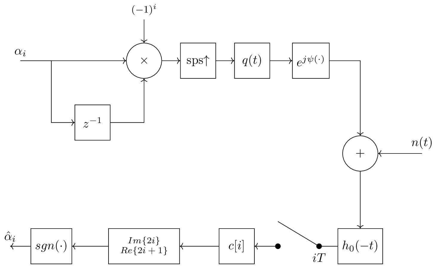
8. Serial Noncoherent Receiver

Previously, it is mentioned that the auxiliary symbols that belong to different PAM component are mutually uncorrelated. However, the same is not the case for the symbols that belong to the same PAM component. The relationship between the original symbols and auxiliary symbols are given in Eq. eq:a_0_n. Naturally, the auxiliary symbols are correlated to each other.

In [3], a method is given to weaken the correlation between the consecutive auxiliary symbols, which should increase the overall BER performance. The idea is basically to increase the depth of differential encoding additionally by employing a complex differential encoder.

A new parameter M is introduced as an odd number, which stands for the total differential encoding depth of the system. The complex differential encoder is as follows:

\beta_i = (-1)^{\frac{M-1}{2}}\alpha_i \prod_{n=1}^{M-1}\beta_{n-1},

Thus M=7 means a complex differential encoder of depth 6 is employed before generating the auxiliary bits and creating the baseband signal. With the addition of the auxiliary bit generation, the total differential encoding depth of the system becomes 7. As a side note, M=1 means no extra differential encoding is done and just PAM receptions inherent differential encoding is present.

In [3], receiver for only odd numbers of M is given. For even M, the decision metric becomes much more complex and is not further explored. Details of the optimum receiver and its decision is also shown there and is not rewritten here.

Since there is differential encoding in the system, this has to be differentially decoded in order to reach the original symbols at the receiver. The total depth of the differential decoder is M.

The block diagram of the transmitter and receiver is in Fig. 3. Here, differential decoder works on the complex signal where as the encoder's input is bipolar NRZ symbols. The gain block only applies -1 or 1, in fact for odd M which is the case in this report and in [3], gain block simply has no effect.

Figure 3. Noncoherent transmitter-receiver block diagram.

9. Conclusion

The corresponding BER curves for various other GMSK receivers and some BPSK receivers is shown in Fig. 4. In the figure, BT = 0.3, M=7, L=3 and K = 30, where K stands for the number of Wiener filter coefficients. As expected, coherent serial receiver, approaches to the BPSK. This is because, PAM representation of GMSK is simply a BSPK type of receiver with some ISI and CSI. As BT increases, both ISI and CSI will diminsh and GMSK will in fact perform as good as BPSK. This can be seen in Fig. 5 where BT=0.5.

Figure 4. Performance of various GMSK schemes for BT = 0.3.

Figure 5. Performance of various GMSK schemes for BT = 0.5.

10. References

[1] Pierre Laurent. Exact and approximate construction of digital phase modulations by superposition of amplitude modulated pulses (amp). IEEE transactions on communications, 34(2):150–160, 1986.
[2] Ghassan Kawas Kaleh. Simple coherent receivers for partial response continuous phase modulation. IEEE Journal on Selected Areas in Communications, 7(9):1427–1436, 1989.
[3] Ghassan Kawas Kaleh. Differentially coherent detection of binary partial response continuous phase modulation with index 0.5. IEEE transactions on communications, 39(9):1335–1340, 1991.
[4] John B Anderson, Tor Aulin, and Carl-Erik Sundberg. Digital phase modulation. Springer Science & Business Media, 2013.
[5] Musa Tunç Arslan. Maximum likelihood sequence detector for gmsk. Technical report, Meteksan Defence Inc., 2018.
[6] Gee L Lui. Threshold detection performance of gmsk signal with bt= 0.5. In Military Communications Conference, 1998. MILCOM 98. Proceedings., IEEE, volume 2, pages 515–519. IEEE, 1998.

Maximum Likelihood Sequence Detector for GMSK

1. Abstract

This report is about the maximum likelihood sequence detection (MLSD) of GMSK scheme. The receiver is done both in coherent and noncoherent means without using limiter discriminator structure or PAM representation of GMSK.

You can find sample MATLAB codes here.

2. Introduction

GMSK waveform can be modeled as both PAM and as a Trellis. Such behavior is beneficial since it enables different receiver structures [1, 2, 3]. A separate serial receiver that exploits the PAM representation of GMSK was examined previously. Both the coherent and non-coherent serial receivers were realized according to Laurent's PAM representation of GMSK and Kaleh's serial receiver [4]. In this short report, MLSD is employed as receiver due to GMSK's Trellis model.

In the following section, necessary mathematical derivations are done in order to write the GMSK waveform's phase as a state machine, ie. some outputs are generated according to some start state. After necessary outputs are generated, the state changes according to a Trellis that is specific to GMSK waveform. In fact, this Trellis structure is not specific to GMSK only but applies to all Continuous Phase Modulation (CPM) schemes.

In the third chapter the MLSD receiver is set so that this Trellis can be solved via Viterbi Algorithm. Unlike regular Viterbi algorithm that is used to solve convolutional coded sequences, this one uses a soft input structure to solve the GMSK Trellis. The regular MLSD receiver is a coherent one. The non-coherent MSLD (NSD) modification is also presented here.

Finally, BER curves are presented with further comments.

3. CPM Waveform as a Trellis

GMSK is a form of CPM. If CPM can be written as a Trellis, GMSK can be as well. CPM waveform has the following structure [1]:
s(t, \underline{\alpha}) = \sqrt{\frac{E}{T}} exp\{j\psi (t, \underline{\alpha})\},
where E is the symbol energy and T is the symbol duration and \underline{\alpha} is a sequence of bipolar NRZ symbols for GMSK. \psi (\cdot) is the phase of the signal which also carries the information. Phase function has the following form [1, 5, 2, 6]:
\psi (t, \underline{\alpha}) = 2\pi h\sum_{i=-\infty}^{n}\alpha_i q(t-iT), \quad nT \leq t < (n+1)T,
where h is the modulation index and h = 0.5 for GMSK. q(\cdot) is the phase shaping filter and is a Gaussian curve for GMSK case. q(\cdot) is defined as follows [1]:
q(t) = \begin{cases}
0, & t < 0, \\ \int_{0}^{t}f(\tau)d\tau, & 0 \leq t < LT,\\ 1/2, & t \geq LT \end{cases}

where f(\cdot) is called the frequency pulse. Here, the integral of the frequency pulse might add up to more than 1/2 when t \ge LT, then q(t) is basically scaled in amplitude. For GMSK, this has Gaussian shape and is calculated via [1]:

f(t) = \frac{1}{2T}\bigg[Q(2\pi B \frac{t-\frac{T}{2}}{\sqrt{ln(2)}}) - Q(2\pi B \frac{t+\frac{T}{2}}{\sqrt{ln(2)}})\bigg],

where B = BT/T, with BT the so called time bandwidth product. Q(\cdot) is the famous Q function.

One important note with Eq. eq:phase_func before going further is that, it is defined for the time interval nT \leq t < (n+1)T when the n^{th} symbol arrives and the phase waveform in Eq. eq:phase_func has a transient shape only in LT duration, which limits the transient curve to L consecutive symbols within the \underline{\alpha}. From another perspective, this is due to the fact that f(\cdot) is only defined in (0, LT_{sym}).

4. Partition of \psi(t, \underline{\alpha})

Phase shaping filter q(t) has variations only within t\in [0, LT]. Looking at the Eq. eq:phase_shaping, when t < 0, q(t) =0, which means \alpha_i, i > n will have no effect on the value of \psi(t, \underline{\alpha}), due to nT \leq t < (n+1)T. On the contrary, \alpha_i, i \leq n-L will have \sum_{i=0}^{n-L} \alpha_i\frac{2\pi h}{2} cumulative effect on the value of \psi(t, \underline{\alpha}). Here, i starts from 0 instead of -\infty since we cannot have infinite amount of symbols. This comes from the way \psi(t, \underline{\alpha}) is defined. Lets now partition \psi(t, \underline{\alpha}) to see aforementioned effect better.

Say, L = 3, N = 5, symbols so, i = 0,1,2,...,5 and n = 4, ie. n=4^{th} symbol just arrived and value of \psi (t, \underline{\alpha}) at \quad 4T \leq t < 5T is of concern:
\psi (t, \underline{\alpha}) = 2\pi h \sum_{i=0}^{4} \alpha_i q(t - iT), \quad 4T \leq t < 5T,
\begin{aligned}
\psi (t, \underline{\alpha}) = 2\pi h\bigg[ & \alpha_0 q(t) + \alpha_1 q(t - T) + \alpha_2 q(t - 2T) \\
& + \alpha_3 q(t - 3T) + \alpha_4 q(t - 4T)\bigg], \quad 4T \leq t < 5T, \end{aligned}
\begin{aligned}
\psi (t, \underline{\alpha}) = 2\pi h\bigg[ & \alpha_0 q(4T \leq t < 5T) + \alpha_1 q(3T \leq t < 4T) \\ & + \alpha_2 q(2T \leq t < 3T) + \alpha_3 q(T \leq t < 2T) + \alpha_4 q(0 \leq t < T)\bigg], \end{aligned}
First of all, q(4T \leq t < 5T) = q(3T \leq t < 4T) = 1/2 since L = 3 and eq:phase_shaping dictates q(t) = 1/2 for t \geq LT. This is the direct effect of the cumulative \sum_{i=0}^{n-L} \alpha_i\frac{2\pi h}{2}. Since L = 3 and n = 4 is chosen. Thus for this case, when n = 4^{th} symbol arrives, \alpha_0 and \alpha_1 has a cumulative and constant effect on the value of \psi (t, \underline{\alpha}).

Furthermore, i=5 is said to have a similar effect, since the time interval of concern is \quad 4T \leq t < 5T, q(\cdot) belonging to the i=5^{th} symbol would be, q(-T \leq t < 0) = 0 due to the way q(\cdot) is defined in Eq. eq:phase_shaping. Thus, it is true that there are 6 symbols that have an impact on \psi (t, \underline{\alpha}). When n=4^{th} symbol arrives, \alpha_i, i \in [0, n-L] have constant cumulative effect whereas \alpha_i, i \in [n+1, N] have no effect, since they are yet to be fed into the system.

Thus, \psi (t, \underline{\alpha}) is partitioned into two parts [2, 6]:

\psi (t, \underline{\alpha}) = \theta(t, \underline{\alpha_n}) + \theta_{n-L},

where,

\theta(t, \underline{\alpha_n}) = 2\pi h \sum_{i=n-L+1}^{n} \alpha_i q(t-iT),

and

\theta_{n-L} = \sum_{i=-\infty}^{n-L} \alpha_i\frac{2\pi h}{2} = \pi h\sum_{i=-\infty}^{n-L} \alpha_i,

Here, nT \leq t < (n+1)T.

Eq. eq:transient is the transient phase that defines the phase curve and is dependent on the L-1 previous symbols that come before n^{th} symbol. This resembles the idea of a start state that consists of L-1 previous symbols, an input at time n and an output is calculated, \psi (t, \underline{\alpha}). Obviously, when the n^{th} symbol comes in, it causes a transition from the start state to an end state. Which awfully sounds like a Trellis.

However, there is also the cumulative value of \theta_{n-L} in Eq. eq:cumulative that needs to be taken care. When n^{th} symbol arrive, \alpha_i, i \in [n-L+1, n] is used to calculate the transient state as per Eq. eq:transient. The previous \alpha_i, i \in [0, n-L] are used to calculate the cumulative state up until to the n-L+1^{th} time. Which is some sort of a separate so called phase state, even though its not actually a state.

In order to visualize this, a small example is as follows; lets assume that BT = 0.3, L = 3, sps = 20. For this case, there are 2^{L-1} = 4 transient states, excluding the aforementioned cumulative state right now. The states, inputs and corresponding outputs are then:

Figure 1. States, inputs and corresponding transient phase curves.These curves are added side by side with the addition of cumulative value calculated via Eq. eq:cumulative. Let us now assume a sequence of symbols flowing:

\underline{\alpha} = [\underset{\underset{n=0}{\downarrow}}{0} 1\, 1\, 0\, 1].

Here, the starting state of the GMSK scheme is [0\, 0], since L=3. First symbol arrives at n=0.

1. First the symbols are converted into bipolar-NRZ such that, 0\rightarrow -1, \quad 1 \rightarrow 1,
2. A sliding window of length L travels along the data, hence at time n=0, the sub-sequence of concern is \underline{\alpha}_{sub} = [-1\, -1\, -1],
3. The cumulative phase is calculated as per Eq. eq:cumulative, for this case, at symbol n=0, cumulative phase is 0 since there are no symbols n-L = -3 yet,
4. The necessary transient phase of this sub-sequence is chosen from Fig. 1,
5. Cumulative phase is added onto the transient phase to calculate the total phase for the time interval of concern.

These steps are done over and over until the data in the sequence finishes. Thus for the symbol sequence of concern, the phase values will be as follows:

Figure 2. Phase curve of the aforementioned \underline{\alpha} sequence.
In Fig. 2, at time n=1, the sub-sequence is, \underline{\alpha}_{sub} = [-1\, -1\, 1] and cumulative phase that is left over from time n=0 is -\frac{\pi}{2}. Thus the curve that corresponds to the sub-sequence is shifted by this value, which can be seen from sample number 21, beginning of the transient phase of the sub-sequence. At time n=2, a similar behavior is apparent, \underline{\alpha}_{sub} = [-1\, 1\, 1] and the cumulative phase that is left over from time n=0 and n=1 is now -\pi, which shifts the transient curve of sub-sequence by this amount. This can be observed at sample 41 and so forth.

Thus the cumulative phase affects the Trellis of CPM scheme and enlarges it.

5. Coherent MLSD Receiver

Received signal is modeled as:

r(t, \underline{\alpha}) = s(t, \underline{\alpha}) + n(t),

where, n(t) is assumed to be AWGN.

The MLSD receiver is intended for finding an \underline{\hat{\alpha}} sequence such that it is closest (in a sense) to the received noisy signal:


\Lambda(\underline{\hat{\alpha}}) = -\int_{-\infty}^{\infty} |r(t) - s(t, \underline{\hat{\alpha}})|^2 dt

An \underline{\hat{\alpha}} sequence that maximizes the Eq. eq:real_metric metric, is the most probable sequence that is transmitted. Maximizing the above sequence for CPM schemes is equal to maximizing correlation [1]:

\lambda(\underline{\hat{\alpha}}) = Re\bigg[\int_{-\infty}^{\infty} r(t)s^*(t, \underline{\hat{\alpha}}) dt\bigg],

Due to the aforementioned Trellis-like structure of CPM signals, the correlation in Eq. eq:metric can be calculated via Viterbi Algorithm (VA).

Using Eq. eq:transient and eq:cumulative, an L-tuple start state can be defined at time n when \alpha_n arrives,

S_n = (\theta_{n-L}, \alpha_{n-L+1}, ..., \alpha_{n-2}, \alpha_{n-1}),

As previously shown, this start state depends on the L-1 \alpha symbols that came just before n^{th} symbol and the cumulative phase that accumulated from the beginning of the data transmission to the (n-L)^{th} symbol. The corresponding end state after n^{th} symbol is then [2, 6]:

E_n = (\theta_{n-L+1}, \alpha_{n-L+2}, ..., \alpha_{n-1}, \alpha_{n}),

The transition from S_n to E_n is done by the following L+1-tuple:

\sigma_n = (\theta_{n-L}, \alpha_{n-L+1}, ..., \alpha_{n-1}, \alpha_{n}).


Combination of these definitions enable a recursive metric update, the metric that accumulated up to n^{th} symbol as follows:

\lambda_{n+1}(\hat{E}_n) = \lambda_n(\hat{S}_n) + Re\bigg[e^{-j\hat{\theta}_{n-L}} z_n(\underline{\hat{\alpha}}_n)\bigg].

Here, e^{-j\theta_{n-L}}is the cumulative phase up until to n^{th} symbol for the hypothetical sequence \underline{\hat{\alpha}}_n and z_n(\cdot) is the sampled matched filter output:

z_n(\underline{\hat{\alpha}}_n) = \int_{nT}^{(n+1)T} r(t)s^*(t, \underline{\hat{\alpha}}_n)dt.


Writing the metric update as in Eq. eq:metric_update enables the opportunity to decrease the number of states from \rho M^{L-1} to M^{L-1} because of the way e^{-j\theta_{n-L}} is calculated. Starting from the first time instant n=0, if the starting state is known a-priori and if e^{-j\theta_{n-L}} is updated when the winner branch up to that time instant, then e^{-j\theta_{n-L}} should have M^{L-1} different values for each time step. Thus each state would have their own "winner" phases that accumulate as the maximum of branch metrics are chosen. Thus, it is not necessary to search for the best of all \rho possible e^{-j\theta_{n-L}} values, but calculating the necessary winner previous state is enough,

\hat{\theta}_{n-L+1}(\hat{E}_n) = \hat{\theta}_{n-L}(\hat{S}_n) + \pi h\hat{\alpha}_{n-L+1}.

This approach decreases the total number of states to M^{L-1} for the Viterbi Algorithm.

6. Noncoherent Receiver

In noncoherent case received signal is modeled as:

r(t, \underline{\alpha}) = s(t, \underline{\alpha})e^{j\phi(t)} + n(t),

where \phi(t) is some time varying phase. In slow fading channels, it can be assumed that \phi(t) = \phi \sim U[0, 2\pi] during the interval in which data is transmitted, which is the case here as well. In such circumstances, the receiver structure also changes. Phase locked loops are common solutions to the random additional phase but they are also expensive.

Thus a noncoherent receiver which has to compensate for the random phase of the channel has to be developed. In the MLSD receiver, the recursive metric calculation in Eq. eq:metric is updated as follows:

\lambda_{n+1}(\hat{E}_n) = \lambda_n(\hat{S}_n) + \bigg[Q^*_n(\hat{S}_n)e^{-j\hat{\theta}_{n-L}} z_n(\underline{\hat{\alpha}}_n)\bigg],

where Q_n(\cdot) is the so called phase reference and is updated via a gradient descent like approach [7];

Q_{n+1}(\hat{E}_n) = aQ_n(\hat{S}_n) + (1-a)\bigg[e^{-j\hat{\theta}_{n-L}}z_n(\hat{\alpha}_n)\bigg].

Here, z_n(\hat{\alpha}_n) is calculated via Eq. eq:correlator, the matched filter output and e^{-j\hat{\theta}_{n-L}} is the same phase update in the coherent receiver. The a parameter is the so called forgetting factor and has the same purpose as in gradient descent approach. As a \rightarrow 1, the system becomes more open to the side effects of the random phase shift, thus becomes "more" coherent. In fact a = 1 is exactly the coherent receiver. As a \rightarrow 0 the opposite happens. Hence, a controls, how much system depends on the current phase as opposed to the previous phase.

7. Example Problem for the Coherent Case

In this problem, it is very important to understand that, if the seed of the random noise is not given same as here, it may not be possible to reach the same results.

Lets assume a sample problem with GMSK, BT = 0.3, L = 3, N = 4 and starting state of [0\, 0], and transmitted symbols \underline{\alpha} sequence is as follows:

\underline{\alpha} = [\underset{\underset{n=0}{\downarrow}}{0} 1\, 1\, 0\, 1].

Corresponding phase function of this symbol stream is in Fig. 2 as previously shown. The reduced state Trellis diagram has 2^{L-1} = 4 states. In this example, system is simulated in MATLAB according to the equations in this report. The SNR is, \frac{E_b}{N_0} = 8 dB and oversampling ratio sps = 20. Noise seed is rng(40) and noise is added via awgn(.) function with 'measured' flag. Thus the noise code snippet becomes:

r = awgn(s, 8-10*log10(sps), 'measured');
The corresponding Trellis is in Fig. 3.

Figure 3. Trellis of the example problem.
In Fig. 3, the winner branch at the end of the process is marked with red. The solid lines correspond to hypothetical input of -1 and dashed lines correspond to a hypothetical input 1. Numbers on the lines correspond to the cumulative metrics as calculated in Eq. eq:metric_update. Cumulative phases that correspond to the phase update as per Eq. eq:phase_update can be seen under the state nodes.

Going backwards in the trellis, the winner path is in Fig. 4. This winner path corresponds to the data sequence of \underline{\hat{\alpha}} = [0\, 1\, 1\, 0\, 1] which is in fact the transmitted data sequence.

Figure 4. Winner path.

8. Conclusion

The corresponding BER curves for various other GMSK receivers and some BPSK receivers is shown in Fig. 5. In the figure, the MSLD based receivers prove to be best among other types when GMSK is of concern even at low BT values such as BT = 0.3. Especially for the non-coherent case the performance of MSLD based receivers are better.

Figure 5. BER results of several different receivers, BT = 0.3.

References

[1] John B Anderson, Tor Aulin, and Carl-Erik Sundberg. Digital phase modulation. Springer Science & Business Media, 2013.
[2] Erik Samuel Perrins. Reduced complexity detection methods for continuous phase modulation. 2005.
[3] P¨ar Moqvist et al. Serially concatenated systems: An iterative decoding approach with application to continuous phase modulation. Lic. Eng. thesis, Chalmers University of Technology, Gothenburg, Sweden, 1999.
[4] Musa Tunç Arslan. PAM Representation of GMSK and Serial Receivers. Technical report, Meteksan Defence Inc., 2018.
[5] Subhashini Gupta, Vikas Bhatia, and LC Mangal. An efficient fpga implementation of gmsk (bt= 0.3) transceiver with non coherent sequence detection for tactical v/uhf waveforms. In Communications (NCC), 2012 National Conference on, pages 1–5. IEEE, 2012.
[6] Afzal Syed. Comparison of noncoherent detectors for soqpsk and gmsk in phase noise channels. International Foundation for Telemetering, 2007.
[7] Lutz Lampe, Robert Schober, and Mani Jain. Noncoherent sequence detection receiver for bluetooth systems. IEEE Journal on Selected Areas in Communications, 23(9):1718–1727, 2005.